The ultimate guide to digital twins for process factories

In this guide we define the term digital twin, discover the important digital twins within a complex supply chain and explore how to create and validate a digital twin for a process factory.

In this guide you will learn:

– The building blocks that make up your broader supply chain.
– The most important elements of a digital twin.
– What digital twins are possible within a complex process industry supply chain.
– The difference between a static and dynamic digital twin
– How to validate a digital twin
– How to monitor the performance of a digital twin.

Scroll down or download the PDF version of this eguide

Click the link to go directly to the heading

Introduction – The 10 high-powered building blocks that change the way you look at your complex supply chain

Step 1 – Identify the 3 prerequisites for a powerful digital twin

Step 2 – Understand the 10 most important digital twins in your process industry supply chain

Step 3 – Create static digital twins for your process factories

Step 4 – Create dynamic digital twins for your process factories

Step 5 – Monitor digital twin performance in your process factories

Step 6 – Monitor digital twin performance for your entire process industry supply chain

Introduction - The 10 high-powered building blocks that change the way you look at your complex supply chain

Ever wish that there were simple, fundamental building blocks that could be used to represent your supply chain, no matter its complexity?

Hidden in the industrial engineering literature are 10 building blocks that can be used to show the performance of an entire supply chain.

When we think of complex supply chains, we often think of terms such as bullwhip effect, advanced planning & optimisation, sales and operations planning, Lean, Six Sigma, the list goes on.

When all the layers are peeled back however, there exists a basic framework that underpins every supply chain and forms the basis on which we can

link the different parts and functions of a business
link the flow of products, materials and resources to the profitability of a business
identify bottlenecks that are hindering the profitable flow of products

The first 4 of the 10 building blocks are primitive building blocks, fundamental elements that exist in all supply chains.

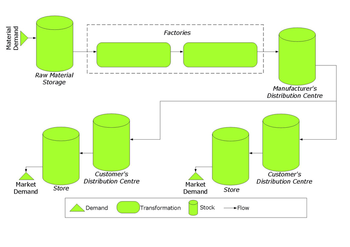
Building Block #1 - Demand

A measure of customer’s desire and willingness to pay a price for a specific good.

Building Block #2 - Transformation

The act of changing materials, or other resources, into goods to meet demand.

Building Block #3 – Stocks

Materials, resources, or finished products waiting for transformation or demand.

Building Block # 4 – Flow

Materials, resources, or finished products moving to, through or from transformation processes or stocks

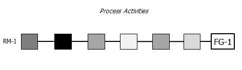
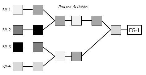
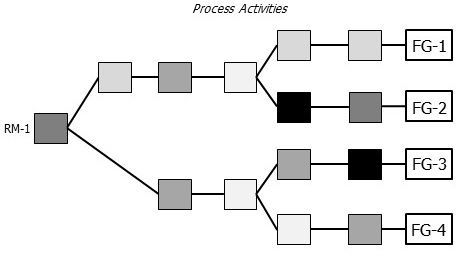
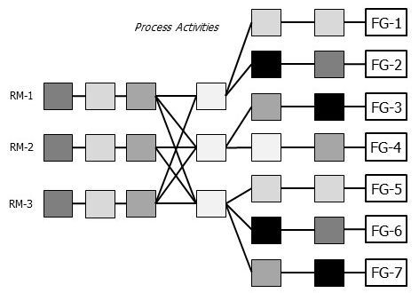
These building blocks can be connected together to represent a supply chain. Here we have a simple retail supply chain.

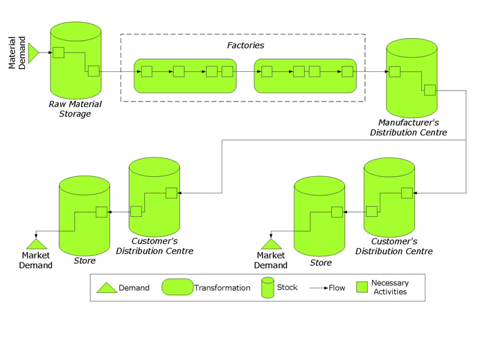
Each transformation process can be split into any number of necessary activities. Also, stock locations such as warehouses involve other necessary activities including a number of unloading, putaway, picking and loading activities.

This brings us to our next building block:

Building Block #5 – Necessary Activities

Necessary activities can be fully manual through to fully automatic activities. These activities can be necessary but non-value adding OR necessary and value adding. In any case they are recognised as necessary activities within the supply chain.

This would be a good and helpful model if demand and transformation behaved in a deterministic way. That is to say, this model would be helpful if we could perfectly predict when a customer wants product and know that factories and resources could transform product with a reliability of 100%. In this case stocks could be restricted to only those required to fulfil particular customer sequencing needs.

However, in the real world:

perfection is impossible, or
if perfection where possible it would be impossibly expensive

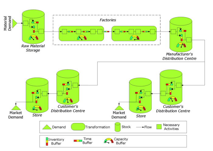
So, to satisfy variable demand using imperfect necessary activities, shock absorbers (or buffers) must be introduced into the system. These behave just like shock absorbers on a car, adjusting to sudden and unanticipated shocks from the road terrain so as to keep the driver safe. In this case we are keeping the customer safe from the uncertainties and shocks that occur in our supply chain.

There are ONLY 3 types of buffers that can be inserted into a supply chain.

Building Block #6 – Inventory Buffer

Extra material between 2 transformation processes or between transformation processes and demand.

Building Block #7 – Time Buffer

Early arrival of material or resources before necessary activities, before transformation processes or before demand.

Building Block #8 – Capacity Buffer

Extra potential capacity in necessary activities or transformation processes needed to satisfy irregular or unpredictable demand rates, otherwise known as “sprint capacity”.

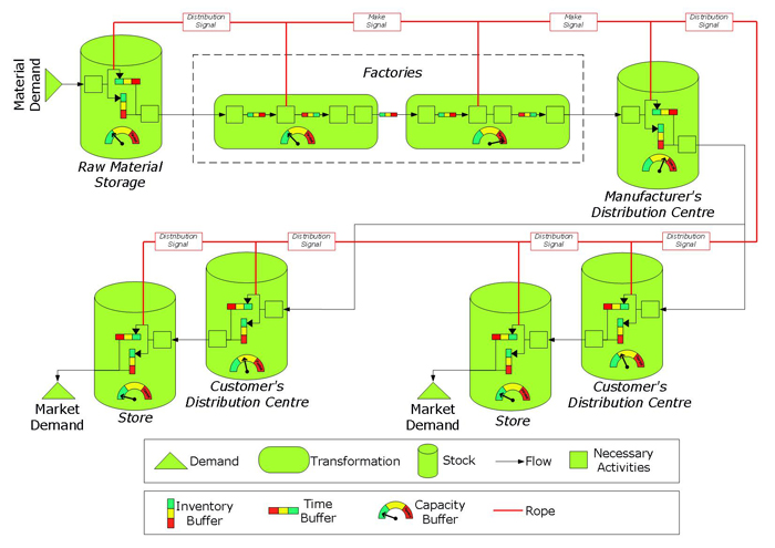
There is more information on buffers in the article Buffers! the secret behind exceptional supply chain performance.

Building Block #9 – Rope

“Rope” is a Theory of Constraints term. It represents the gating mechanism used to manage make and distribution signals within a supply chain.

These building blocks can be used to represent a supply chain and it’s not too hard to think of a way we could animate this conceptual framework. We could use colour coded meters and gauges to represent flow, the depletion of stocks and the flexing of buffers. This would create a compelling show and mesmerise us as we witnessed a complex adaptive system in motion.

The performance of the system could be measured by how frequently different buffers got to dangerous levels. This would be helpful but it would fail to do two things;

identify when we miss supply obligations completely
identify specific bottlenecks that cause supply disruptions

To do this a final piece of the puzzle must be introduced.

Building Block #10 – The Control Point

Control points are placed before and after time buffers or inventory buffers. They measure the frequency with which products, materials or resources were unavailable at crucial points within a supply chain.

These building blocks can be used to represent any supply chain. Why is this helpful?

These 10 building blocks are the essential elements of Value Stream Maps for the process industry. They provide a means by which planned structural modifications to a supply chain can be represented; communicating the impacts on flow by using a current state map and a future state map. When combined with financial data, showing total-cost-to-serve, this provides a more comprehensive view of supply chain improvement proposals.
The building blocks provide a skeleton on which the flesh of data can be hung. We can choose to introduce data to all the building blocks or we can take a more forensic approach, using data to confirm our perception of how we think the supply chain is operating at a specific point.
Together the building blocks provide a systemic view of the supply chain. For example, while minimising the size of all the buffers is important (i.e. Lean), its important that buffer sizes are only reduced with an understanding of how the changes will impact the rest of the system.

Having introduced the building blocks of supply chains we now turn our attention to identifying the most important operational leverage points in a complex supply chain.

Step 1 - Identify the 3 prerequisites for a powerful digital twin

Digital twins are simply the digital clone of a system.

Digital twins in the supply chain take many forms; from animated dynamic models that show factory behaviour to the digital scorecards used to control corporate-wide supply chain performance. Digital twins can be a spreadsheet, a CAD drawing, a sophisticated business proposal or a complex dynamic simulation.

The common characteristic is that the twin is digital, and it accurately depicts the behaviour change or state change of a system during the achievement of a business goal.

Digital twins are expensive so there are 3 prerequisites that must be met before creating a digital twin in the service of an important business goal.

The goal must be worth it

We believe there are 3 parts to defining robust business goals for operations.

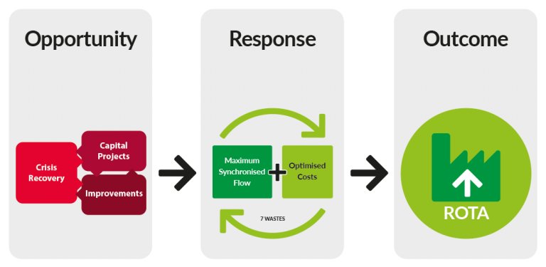
Opportunity

There are always 3 types of opportunity within a supply chain as shown above: Crisis Recovery, Capital Projects, and Improvements.

There are plenty of targets, and this is always the case in the process industry. Combine this with the fact that there are less humans in the process industry to do the work then it is easy to see why opportunities should be prioritised.

Response

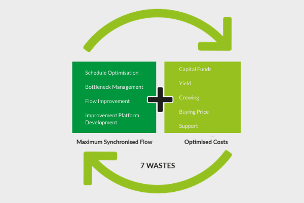
The response to any opportunity (above) should support a virtuous circle in which synchronised flow is being maximised, costs optimised and waste minimised (see graphic below).

The table below shows more detail on Synchronised Flow in a process factory.

Notice that traditional continuous improvement frameworks form only part of a robust improvement platform from which broader business improvements can be added and sustained. This is something of a paradigm shift!

There have been many cases where the number of opportunities has increased because of a poor response to a previous opportunity.

For example, a buyer tries to minimise (not optimise) buying price by reducing the quality of raw material inputs (a distortion of what was originally a good opportunity) which causes a reduction in processing machine performance. This increases crewing costs, increases support resources (e.g. maintenance costs) and reduces yield (all together reducing synchronised flow). This increases the number of opportunities in the supply chain as well as causing a net reduction in business performance (reducing ROTA).

Selecting a good response to an opportunity within a complex processing factory is sophisticated. Done well it creates a virtuous circle that exceeds expectations. Selecting a poor response to an opportunity almost always causes a net reduction in business performance and leaves an insidious weakness in the operating system.

A ranking of a business opportunity should always be measured assuming the resources that will be needed to deliver the right response not the most expedient response.

Outcome

In the end, the success of a business is measured by Returned On Total Assets (ROTA).

When prioritising opportunities, the final arbiter should be ROTA. The projected ROTA should be assessed while taking into consideration the most effective (not expedient) response.

I can hear the advocates for corporate responsibility (e.g. safety, environment, etc) crying foul here! Perhaps there is an additional measure apart from ROTA or you could just argue for a longer view of ROTA.

The goal must be capable of being modelled

Digital twins must be based on a model. For the model to be a digital twin it must represent reality.

Modelling the behaviour of sections within a supply chain, with reference to reality, forces a business to consider what is really happening. A model of the current and future state of a system, in today’s high technology world, must take account of 3 important factors:

Variability (controlled using buffers)
The key variables that effect performance
How targets for the future state can be achieved

There are many types of models within a supply chain and we have listed 10 of the most important below. The key is to know when and how to apply these different modelling techniques within a supply chain.

Demand modelling
Network modelling (node positioning using linear programming tools)
Dynamic transport modelling (using statistical analysis and queue theory to demonstrate the time-based behaviour of a transport system)
Inventory buffer sizing (using different order size and variability factors to determine optimum inventory levels)
Financial modelling – projects and project risks
Value stream mapping
Factory schedule modelling
Factory constraints and capacity modelling
3D Computer Aided Design (CAD) models
Dynamic factory modelling

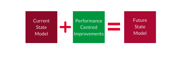
A model is used to define:

what is expected to happen now (Current State)
what is possible into the future (Future State)
how to get from the current state to the future state (Performance Centred Improvements)

The goal must be capable of being monitored

The way a system was modelled determines the way it must be monitored. If the monitoring method in the ERP system does not manage the key variables identified in the model, then it simply is not suitable.

A monitoring system shows how the current performance of a system is deviating from that which was expected in the model. The monitoring system should:

show how buffers (inserted into the system to manage variability) are performing
focus attention on prioritised performance centred improvements (see above)
demonstrate progress towards a modelled future state

IF monitored behaviour = monitored behaviour then you have a powerful digital twin!

Finally, like all good adaptive and improvement systems there needs to be a feedback loop. Business priorities change so the modelling and monitoring activities, that together form the digital twin, should be adjusted accordingly.

Step 2 - Understand the 10 most important digital twins in your process industry supply chain

At our last count we reckon there are 10 digital twins in a process industry supply chain.

Demand modelling
Network modelling
Dynamic transport modelling
Inventory buffer sizing
Financial modelling – projects and project risks
Value stream mapping
Factory schedule model
Factory constraints and capacity model
3D Computer Aided Design (CAD) models
Dynamic factory modelling

The first 6 appear in all supply chains.

The last 4 are more specific to factories in the process industry.

They are all digital twins to the extent that they rely on digital techniques (e.g. excel spreadsheets through to Artificial Intelligence) and they are designed to replicate (or twin) reality.

We will deal with supply chain digital twins (1 to 6) in this Step and the other factory-based twins (7 to 10) in Steps 3 and 4 below.

1 - Demand Modelling

In the introduction we went through the 10 building blocks of a supply chain as summarised below.

Demand modelling is complex. That complexity is amplified as you measure demand at Control Points that are further away from the actual Market Demand as shown above.

Very complex “flow casting” and statistical methods can be deployed to try and control and regulate the flow of information through the pipeline but this is becoming unmanageable due to the changing nature of Market Demand in an increasingly unpredictable world.

Businesses are turning to adaptive systems that can be plugged in at any Control Point within a supply chain. These systems rely on averages and factors for medium to long term planning and Artificial Intelligence or “demand driven” adaptive systems for short term planning (see Demand Driven approach to inventory buffer sizing below)

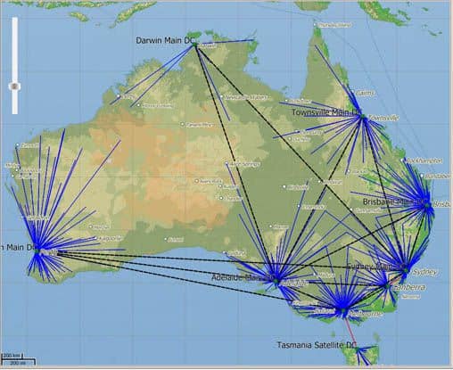
2 - Network modelling

The discipline of supply chain network design is used to determine the optimal location and size of facilities and the optimal flow through the facilities.

Up to 80% of the costs of a supply chain are determined by location of the facilities and the flow of product between them.

Companies that have not evaluated their supply chain in several years, or those that have a new supply chain through acquisitions, can expect to reduce long-term transportation, warehousing, and other supply chain costs from 5% to 15% by reviewing their network design.

However, the problem with network design is that it is complex.

There are many consultants capable of performing supply chain network design and optimisation. They use different software packages to do the analysis (one of the most popular being Lamasoft).

These packages are developed in the context of very sophisticated supply chains and so the requirements of an Australia-wide network analysis are well within the capabilities of these packages.

The aim of the package is to come up with the optimum location of distribution nodes that minimise certain target criteria such as transport cost.

The core of these software packages is mathematical optimisation relying on linear and integer programming. These techniques have been around since the invention of the computer. That said, developers such as Lamasoft augment their software capability with Artificial Intelligence and very accurate mapping information.

3 - Dynamic transport modelling

There are 2 types of modelling used in the transport industry to understand the behaviour of trucks, ships and the people that pilot them. They are:

Agent based
Discrete event

At Bullant Creative we specialise in the use of 3D discrete event simulation software for factory-based dynamic modelling. Discrete event simulation is used in complex systems where the behaviour of resources within that system are predictable using statistical assumptions.

We can use this same software to simulate the behaviour of trucks and resources in supply chains and at warehouses or factories.

Agent based simulation is a technique that can consider the unusual behaviour of the individual resource (agent) within a system. It is more capable of considering things like the variable reaction of individual ships to storms, the response of drivers to road closures or even the passage of disease throughout a population.

The leaders in the area of agent based modelling (or discrete event simulation that relies an accurate mapping database) are a company called Anylogic.

4 - Inventory buffer sizing

Inventory buffers are used to manage Make-To-Stock products and materials. Time buffers and capacity buffers are used to manage Make-To-Order products and materials.

Inventory buffers are used to absorb demand and supply variation for those finished goods, raw materials and parts that have a high average demand relative to the optimum replenishment quantity.

The intention of an inventory buffer is to decouple the downstream customer or process from upstream lead times and variability. We can size inventory buffers using the following approaches which generally involve some excel-based desktop work at the Stock Keeping Unit (SKU) level:

5 - Financial modelling - projects and project risks

Financial modelling has been around for a long time.

Capital projects within the process industry are particularly reliant on robust financial modelling, often with a requirement for complex Monte Carlo simulation to model the probability of different outcomes.

There are now sophisticated financial modelling techniques that can model the financial behaviour of complete supply chain demonstrating the financial consequences of different future state scenarios.

6 - Value stream mapping

Value stream maps are a great way of summarising and communicating the behaviour of supply chains and factories.

Made popular by the Lean movement in the 80’s, value stream maps rely on computers and analysis frameworks to display the pictorial representations and to demonstrate accurate information.

The traditional value stream mapping approach must be modified for the process industry, incorporating buffers and control points as described in the introduction.

There are also 2 levels of value stream maps:

the supply chain level
the factory level

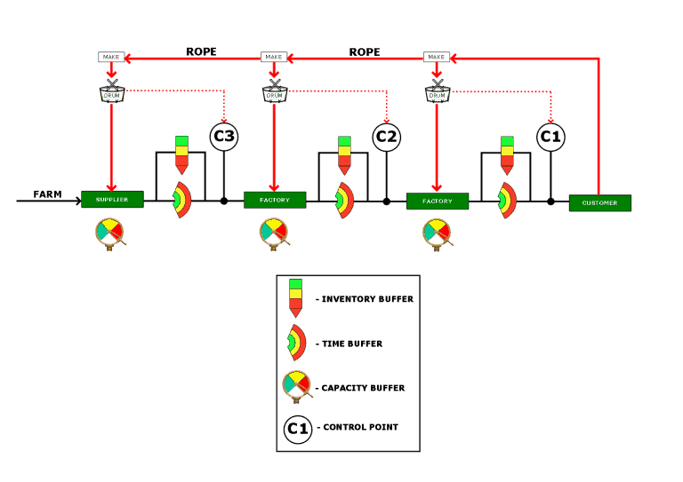
Supply chain level value stream mapping

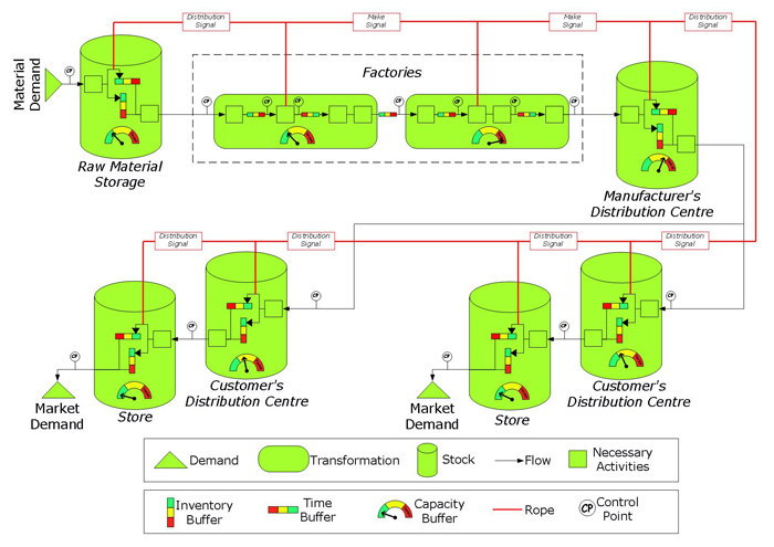
A Value Stream Map at the supply chain level is used to visually represent a total end-to-end supply chain. A simplified schematic is shown below.

The biggest issue with most supply chains is that each buffer is controlled by different people or departments. Consequently, buffers fight against each other as the people controlling them strive for different, localised, performance outcomes.

Maximum flow for the supply chain is only achieved when the performance of each buffer is monitored and adjusted according to the needs of the entire supply system.

The measure of success with this Value Stream Map, is the positive impact it has on the ROI. To achieve this, improvements are identified on a Future State map. Metrics identified in a supply chain level Value Stream Map include:

- - Lead time
  - Inventory Turns
  - Inventory carrying costs
  - Perfect-order execution
  - Demand Amplification
  - Quality Performance

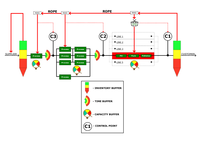
Factory level value stream mapping

A simplified factory level Value Stream Map is shown below.

For high technology process industries, the drum of the supply chain is located at the company-owned, or 3rd party, factory. The successful operation of the supply chain is determined by how well buffers are regulated upstream and downstream of the drum to maximise the flow of raw materials and finished product to the customer.

Step 3 - Create static digital twins for your process factories

Static digital twins are models that rely on averages. If variation must be taken into account, then it can be accounted for using static buffer allowances.

In this way static digital twins can be created using spreadsheets or Computer Aided Design (CAD) software that require only basic programming or statistical manipulation.

There are 3 types of static digital twins in a process factory:

Factory schedule model
Factory constraints & capacity model
3D Computer Aided Design (CAD) model

Factory schedule model

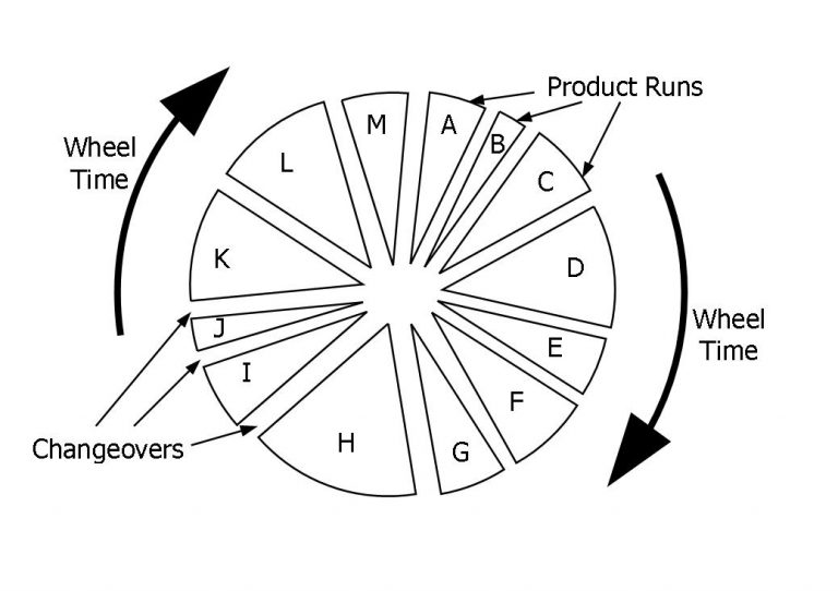
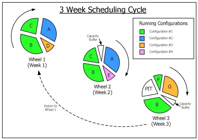
Product portfolios in the process industry are complicated. Paradoxically this makes it easier to model a recurring scheduling cycle for a given production line. The model can then be used to check the extent to which the balance (above) is being achieved.

Generally, complex products must run on a single bespoke processing line. There is always a logical way to order these product runs.

If the average demand for each product is also calculated it becomes a matter of desk work to create several weekly cycles as shown below.

These are known as Product Wheels and in the process industry there are usually 3 or 4 weekly Product Wheels in a standard recurring scheduling cycle.

The optimum Product Wheel sequence for a process factory is one in which there is a balance between:

the cost of changeovers,
the cost of inventory and,
the level of customer service.

Factory constraints & capacity model

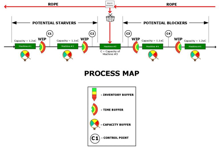
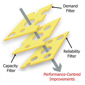
We simply could not find a consistent and comprehensive way of modelling constraints or capacity in the process industry, so we came up with our own system which we called the Bullant Filters.

The Bullant Filters are used on the flow lines commonly found in the process industry where the bottleneck (the Drum) is resident within a group of interconnected and automated workstations, as shown below.

Like the alignment of holes in swiss cheese slices, an issue identified in all 3 filters is a Performance-Centred Improvement opportunity that can add the maximum value.

Watch this short video which explains how the Bullant Filters are a comprehensive way of modelling constraints and capacity on a process line.

Computer Aided Design (CAD)

3D CAD software is becoming more versatile and powerful. There are now 3D sketching tools that can be used to design complete factories with very little drain on computer power.

There is also software at the other end of the spectrum that can incorporate exceptional detail, identify clashes, and animate installation sequences.

In any case the power of CAD is its ability to confirm the 3D design of full processes minimising problems during installation and commissioning.

Step 4 - Create dynamic digital twins for your process factories

Dynamic digital twins rely on the most sophisticated of modelling techniques used in process factories.

Dynamic twins are used when the buffers required for sequencing and efficiency are impossible to size using basic software such as excel spreadsheets.

But first we need to provide some information on plant types and buffers before we get into some examples of dynamic models.

The four plant types

There are 4 plant types in factories, although these types can be combined in many ways. Car factories and assembly plants are predominantly A-Plants and factories in the process industry are mostly I-Plants, V-Plants or T-Plants as shown below

I-plant – Material flows in a straight sequence of events (one-to-one). There are generally as many inputs as outputs. The capacity is determined by the slowest operation known as the Bottleneck, the Capacity Constrained Resource (CCR) or the Drum. These are known as Flow Lines.

A-plant – The general flow of the plant is many-to-one, such as a plant where many sub-assemblies are converging for a final assembly. The primary problem in A-plants is synchronising the converging lines.

V-plant – The general flow of material is one-to-many, such as a plant that takes one raw material and can make many final products. V-plants are most common in the process industry. Examples are meat rendering plants, rice plants, or steel manufacturers. The biggest issue with V-plants is “robbing” where on operation immediately after a diverging point, steals materials meant for a different product or operation.

T-plant – reflects a limited number of components that can be assembled in a wide variety of ways to create a very large number of finished products. T-plants suffer from both the synchronisation problems of A-plants (parts aren’t available at the converging lines) and the robbing problems of V-plants (one assembly steals parts that could have been used in another).

Buffers

Buffers are inserted within these plants to manage the unique challenges of each plant type.

There are 3 types of buffer.

Time buffer
Capacity buffer
Inventory buffer

The main aim of the buffers is to ensure that downstream resources are not starved and that efficiencies throughout the plant are maximised.

Here is an example of an actual T-plant with buffers and control points (see the introduction for more information on buffers and control points).

Dynamic twins

In the example shown in the preceding graphic, Line 4 was out of capacity and information from control point C2 indicated that the line was regularly starved of product.

Attempts had been made to model this system using Excel however they had failed.

This system was modelled (i.e. a digital twin created) using our discrete event simulation tool.

This digital twin could only be a success if it showed the behaviour of metrics that related to the business goal (see Section 1) in this case the running efficiency on Line 4.

The model showed that poor sizing and design of the buffer capacity had translated into product starving and therefore poor performance for Line 4. The model also helped to identify different options for a solution.

Limited excerpts from that model are shown below for information while adhering to NDA requirements.

In another T-plant, a capital plan was being developed to replace the cookers in the centre of the factory.

The client wanted to know if he needed to purchase 5 expensive cookers or 6 cookers to achieve the performance requirements of the total factory. He also wanted to know the storage and labour requirements for each scenario.

Limited excerpts from that model are shown below for information while adhering to NDA requirements.

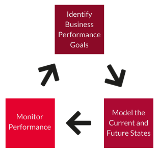
Step 5 - Monitor digital twin performance in your process factories

A digital twin is used to accurately depict the behaviour change or state change of a system during the achievement of a business goal.

The goal must be:

worth it (Step 1)
capable of being modelled (Steps 2 to 4)
capable of being monitored

In Step 1 we defined a framework for identifying the value of goals within a process factory.

In Steps 2, 3 and 4 we have introduced the 10 different modelling techniques available within a process industry supply chain.

The models are used to define a current state and a future state. The difference between these 2 states represents the changes that will take place because of completing the Performance Centred Improvements (shown below).

The goals (i.e. increases in ROTA) are achieved by completing the Performance Centred Improvements.

If all of this is true, then the Performance Centred Improvements will deliver an increase in ROTA (if not then go back to Step 1).

The ROTA increase delivered by the Performance Centred Improvements will be:

A measure of cost
A measure of the 7 wastes
A measure of synchronised flow

or a combination of all 3, as shown below.

Notice that in this section we have yet to call the models digital twins.

The only way we can call a model a digital twin is if that model has been validated against reality (i.e. the digital model is the twin of reality).

To validate a model against reality we must be able to confirm the following:

That the ROTA-based metrics that determine the success of the Performance Centred Improvements (above) can be monitored
That the current state version of the model can demonstrate the behaviour of these ROTA-based metrics during all the necessary operating scenarios
That the behaviour of the ROTA-based metrics in the current state version of the model matches the monitored behaviour of the ROTA-based metrics in the real world.
That the future state version of the model shows an improvement in ROTA-based metrics and, that this improvement matches that which was expected because of the Performance Centred Improvements
That the differences between the current state and future state models is achievable.
That the transition from the current state to the future state can be monitored.

As you can see, monitoring ROTA-based metrics is a crucial part of validating a digital twin.

Of the 3 ROTA improvement measures described above (i.e. costs, the 7 wastes and synchronised flow), synchronised flow is the most poorly understood and therefore poorly monitored.

The table below shows more detail on synchronised flow for a process factory.

While complex automated recording systems in process factories can help with the achievement of the Performance Centred Improvements, they are not necessary for monitoring the ROTA-based metrics associated with synchronised flow.

All you need in to monitor the ROTA-based metrics for synchronised flow is the actual finished product (e.g. cartons) production data for each item and run.

We have developed a simple Bullant Performance Monitoring System (BPMS) to provide all the monitoring information needed to validate models in relation to synchronised flow.

BPMS requires only 4 inputs for each product run making it simple and fast for plant schedulers to update and maintain.

Here is a short video showing some of the BPMS interfaces.

Step 6 - Monitor digital twin performance for your entire process industry supply chain

Finally, if our approach to digital twins is solid then we should be able to come up with a way of monitoring an entire process industry supply chain.

In this video we provide a scenario in which a senior supply chain manager is dealing with a crisis.

This video demonstrates how all the elements described in this guide can be used to monitor an entire supply chain.

We have called the monitoring tool a Flow Console in this video, but you can choose any name you like. Supply chains in the process industry are so complex and dynamic that the high-level monitoring system must be tailor-made.