What is the Lean approach to inventory buffer sizing?

The Lean ethos is that all inventory is evil. “Inventory is one of the 7 wastes so it must be bad!”

Yes it is bad if it is hiding waste such as over-production or under-production. If, on the other hand, an inventory buffer is cost effectively protecting the customer from surges in external demand as well as supply variation and instability then it is adding value.

The management of inventory buffers using forecast-driven MRP systems usually starts with the definition of minimum and maximum stock levels. These stock levels are often calculated on the basis of days of supply and try to fulfil the competing tensions of;

1. assuring the minimum of stock-outs for the customer, and
2. minimising inventory costs and handling charges.

The system is then managed using forecasts, BOM’s and frequent MRP explosions.

In this environment though, neither maximum customer service nor minimum inventories is actually achieved. In fact scrap rates due to product spoilage or obsolescence remain frustratingly high caused by an ever-present bi-model inventory distribution;

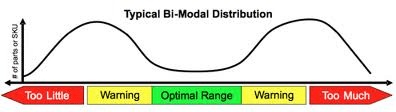
This is caused by, what seems like, an insurmountable number of roadblocks;

• Long replenishment lead times
• Unreliable factories or vendors
• Inaccurate forecasts
• Inaccurate BOMs
• MRP “nervousness”
• The “bullwhip effect”

Lean practitioners know that all forecast-driven MRP systems are push (not pull) systems. These systems can be made more reliable using sophisticated forecasting algorithms, better BOMs, more robust procedures, etc but in today’s complex supply chains this is becoming harder to achieve and sustain.

The Lean approach towards inventory sizing and management sets out to shield the customer from these weaknesses by customising inventory size for each product and material based on;

• customer service targets
• historical demand information
• historical variability information

This approach is known as a Plan For Every Part or PFEP.

Inventory levels are then restored to the calculated levels according to actual demand and this is a key characteristic of a pull replenishment system. Forecast-driven MRP systems on the other hand replenish material without regard to inventory status (and this is a push strategy)¹.

The trick is to figure out how much inventory buffer is just enough to protect the customer. To explain this, we rely heavily on the following Lean Enterprise Institute resources;

• Creating Level Pull Pull by Art Smalley
• Building a Lean Fulfillment Stream by Robert Martichenko & Kevin von Grabe

This is not because we couldn’t create an explanation based on our own experiences and ideas, its just that we want this to be more of a purist’s view of how to design a Lean inventory buffer. We also wanted to make sure that we clearly credit these books as the origin of the graphics and table shown below.

Calculating the size of an Lean inventory buffer

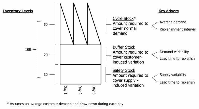
The sizing of a Lean inventory buffer is determined by 4 key drivers;

1. Average demand
2. Replenishment interval (based on an optimum order quantity)
3. Lead time to replenish
4. Demand variability
5. Supply variability

These drivers are then analysed to arrive at the sizing for 3 different components of the total inventory buffer;

1. Cycle Stock
2. Buffer Stock
3. Safety Stock

as shown in the graphic below.

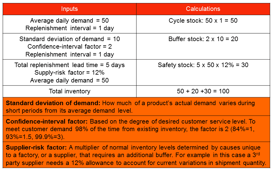
The calculations used in this example are shown below;

Reducing the size of a Lean inventory buffer

This can be achieved in 3 ways;

1. Replenishment Lead Time Reduction – bring factory/supplier/warehouse closer to the demand or modify scheduling sequence at the factory/supplier.
2. Variability Reduction – improve factory/supplier delivery performance or restructure network to increase effects of stock aggregation.
3. Replenishment Interval Reduction – increase delivery frequency from warehouse or increase changeovers at factory/supplier

Key weaknesses for a Lean inventory buffer

There are 2 key weaknesses with sizing an inventory buffer using the Lean approach;

1. it is exposed to unforeseen size creep due to changes in the supply network such as mix changes, changes to product deployment rules from warehouses, etc
2. it fails to take a view on the statistical benefits of different inventory positioning alternatives.

Notes:
¹ The original order quantity and timing of orders calculated using forecast-driven MRP may be close to that derived from the Lean approach. The difference is that a forecast-driven system will prioritise the computer-generated order over the most current inventory status. This can cause significant over or under production/supply and is often the root cause of bi-model inventory distribution.