
Activity Based Costing (ABC) has replaced older methods of cost accounting. Overheads are apportioned to products on the basis of how much of the overhead activities are actually required by the product.
However, when comparing options for operational change we use Contribution Margin or Octane rather than Unit Cost (whether unit costs are derived from ABC models or other older accounting methods). In this article we provide examples of why using Contribution Margin or Octane is a better approach when comparing future operational states.
To illustrate our approach of using Contribution Margin or Octane rather than Unit Costs for operational comparisons we have used examples from two books; “Manufacturing at Warp Speed – Optimising Supply Chain Financial Performance”, by Eli Schragenheim and H. William Dettmer, CRC Press 2001, and “Factory Physics for Managers: How Leaders Improve Performance in a Post-Lean Six Sigma World”, by Edward S. Pound, Jeffrey H. Bell and Mark L. Spearman, McGraw-Hill 2014.
WE ARE NOT suggesting that 100’s of years of accounting practice is now defunct. We just believe that the methodology here is more useful when comparing future operational states. Once the operational strategy has been decided then ABC costing can be used to ratify the decision relative to the broader business context (and this is entirely appropriate from a good business governance point of view).
The examples below are for two different scenarios; 1. Opportunity for greater volume at lower price, and 2. Comparison of product choices on a constrained line. These are very simple examples and we know people will say “that’s too theoretical!” however the logic is sound and it is good theory because it predicts behaviour.
Opportunity for Greater Volume at Lower Price
The sales department says that it can get a very large order but at a 5% reduction in price and we need to decide quickly.
The product sells for $88 per unit. Variable cost is $45 per unit. Fixed company overhead (including direct and indirect labour) is $6000 per week. The forecast sales demand (without the new order) is 150 units per week.
Traditional cost accounting would say, “Subtract the $45 variable cost from the unit selling price (revenue), then allocate part of the total overhead against each unit of product forecast to be sold ($6000 divided by 150 = $40 per unit). Subtract the $40 of overhead allocated to each unit, and the gross profit per unit is $3.00.”
| Traditional Cost Counting | Decision Support with Contribution Margin |
|
| Revenue | $88 | $88 |
| Variable Cost | $45 | $45 |
| Overhead Allocation | $40 | N/A |
| Gross Profit | $3 | N/A |
| Contribution Margin | N/A | $43 |
Decision making using Contribution Margin would say, “Subtract the $45 variable cost from the unit selling price (revenue),and the Contribution Margin is $43.00 per unit.” However, remember Contribution Margin is not the same as net profit. What happens to the overhead costs when using Contribution Margin for the decision process? Hold that thought -we’ll see the answer to that question in just a minute.
Let’s say that the market currently demands 150 units of the product per week, and our new customer wants 50 more than that at the 5% reduced price. If we have the capacity to deliver this order without buying more machines or adding employees or overtime, will we make or lose money on the order.
First, let’s compute the answer using traditional accounting procedures (see table below). If we grant the 5% price reduction, our new selling price is $83.60. Variable cost doesn’t change, it remains at $45.
Overhead allocation doesn’t change either, it’s still $40 (ABC costing allocations are usually changed/adjusted for the aggregate planning process – maybe not until next year). If we subtract these two from $83.60, we get minus $1.40. Multiplied by the 50 additional units we’d be selling at the reduced price, we come up with a $70.00 loss! Definitely, we’d reject this order!
| Selling Price | $83.60 |
| Variable Cost | $45.00 |
| Overhead | $40.00 |
| Profit per Unit | -$1.40 |
| No of Units in the New Order | 50 |
| LOSS on the New Order | -$70.00 |
Now let’s see what the difference is if we calculate the answer using throughput (Contribution Margin) accounting procedures (see table below) and for this very simple example we will assume that the line has plenty of capacity and that no other products are produced on the line (this situation is dealt with in the next example).
If we subtract the $45 variable cost from the new reduced price of $83.60, we find that our Contribution Margin is $38.60. We know we have a current market demand for 150 per week at $88 each, and we won’t be obligated to reduce the price on those deliveries.
Our new customer wants another 50 per week at $83.60. Our total Contribution Margin for existing demand is $6450 ($88-$45 = $43, and $43 x 150 = $6450). Our Contribution Margin for the potential new order is $1930 ($83.60-$45 =$38.60, and $38.60 x 50 = $1930). So the combined projected Contribution Margin for both is $8380.
Now, remember that fixed overhead is $6000 per week, and we don’t spend any more for additional machines, people, or overtime, because we already have the capacity to produce those additional 50 units.
So, since we incur no additional operating expense, if we don’t accept the order, our current net profit (Contribution Margin minus Operating Expense) doesn’t change. It’s only $6450 -$6000, or $450.
But if we do accept the order, our projected net profit will be $8380-$6000, or +$2380! In other words, we forego $1930 in additional profit if we base our decision on traditional accounting and unit costs alone. In other words we pass on an opportunity to increase our profit by more than four times!
| Selling Price | $83.60 |
| Variable Cost | $45.00 |
| Contribution Margin | $38.60 |
| Current Market Demand | 150 Units per Week |
| Potential New Order | 50 per week |
| Contribution Margin for Existing Demand (150x$43.00) | $6,450.00 |
| Contribution Margin for Potential New Order (50x$38.60) | $1,930.00 |
| Total Projected Contribution Margin | $8,380.00 |
| Less Fixed Overhead (Operating Expense) | -$6,000.00 |
| Net Profit (with new order) | $2,380.00 |
| Net Profit (without order = 150x$3) | $450.00 |
| Increase in Profit | 430% |
Comparision of Product Choices on a Constrained Line
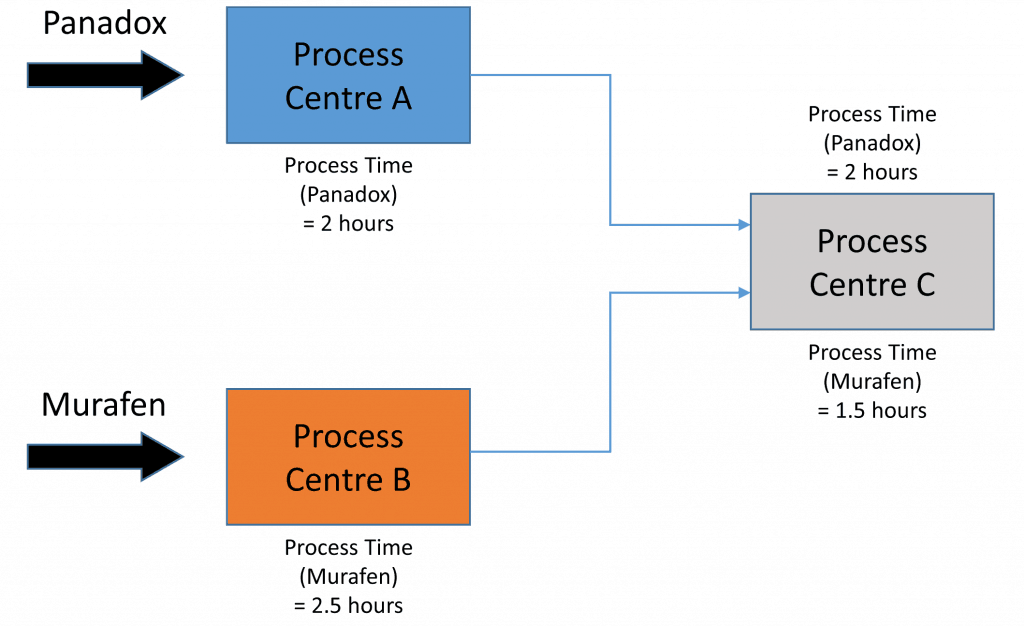
Now consider the example of a pharmaceutical company with two products, Panadox and Murafen. The routings for both products are shown below. A unit of Panadox requires 2 hours of process time at process centre A and 2 hours at process centre C. A unit of Murafen requires 2.5 hours of process time at process centre B and 1.5 hours at process centre C.
The per unit cost elements of the two products are shown below;
| Product | Price | Raw Material Cost | Total Labour Hours | Unit Cost |
Minimum Demand |
Maximum Demand |
| Panadox | $625 | $50 | 4 | $130 | 75 | 140 |
| Murafen | $600 | $100 | 4 | $180 | 0 | 140 |
Labour Charge = $20/hour
Crewed Time = 336 hours per month (at each process centre)
Overhead = $100,000 per month (which includes labour)
| Contribution Margin (per unit basis) |
Contribution Margin /Labour Hr |
|
| Panadox | $575 | $144 |
| Murafen | $500 | $125 |
A manager might evaluate the profitability of potential product-mix strategies by looking at the contribution margin on a per unit basis without regard to how much contribution margin can be produced by the bottleneck.
In this scenario, it would seem that a manager should maximize the amount of Panadox produced because it has the highest contribution margin on a per unit basis. Note that in the “Minimum Demand” and “Maximum Demand” columns, the marketing and sales department has placed limits on the amount of each product that can be produced per month based on its sales forecast.
So, on the basis of these figures the production department naturally wants to make as much Panadox as possible because the contribution margin (on a per unit basisi) shows it to be the most profitable product.
Thus, if we produce the maximum amount (140 per month) of Panadox, we have only enough capacity left over to produce 37 units of Murafen at Process Centre C. The results are shown below. The results are not good; the manager loses $1,000 per month.
| Amount (units) |
Contribution Margin |
|||
| Panadox | 140 | $575 | $80,500 | |
| Murafen | 37 | $500 | $18,500 | |
| $99,000 | ||||
| -$100,000 | ||||
| -$1000 | Profit per Month |
However, because the manager is aware of some fundamental Industrial Engineering principals and thereby the importance of time at the constraint in controlling output, his focus shifted to contribution margin at the constraint.
First, the manager has to figure out which process center is the constraint. Looking at the routing figure above, the initial reaction might be that process center B is the constraint because it has the longest process time (2.5 hours).
However, the manager knows that the process center with the highest utilization is the constraint. Looking again at the figure and the data, it is obvious that process center C is in fact the constraint because both products pass through it. Given the demand mix of Panadox and Murafen, process center C will run out of capacity before any of the other process centres do.
So now the manager does a simple calculation, divides the contribution margin of each product by its time on the constraint, the resulting figure is known as Octane, and the manager calculates the following:
Panadox Octane = (625 – 50)/2 = $287.50 per hour on the bottleneck
Murafen Octane = (600 -100)/1.5 = $333.33 per hour on the bottleneck
This is an eye opener. It turns out the Murafen is the big earner from the perspective of the plant bottleneck and in terms of the time-based recovery of costs.
If the manager wants to generate the most cash possible for the company, he will make the minimum allowed amount of Panadox, because that is what marketting and sales directed, and dedicate the remaining capacity to Murafen. The result of this strategy is shown below and the results are good, the company makes a profit.
| Amount (units) |
Contribution Margin |
|||
| Paradox | 75 | $575 | $43,125 | |
| Murafen | 124 | $500 | $62,000 | |
| $105,125 | ||||
| -$100,000 | ||||
| $5,125 | Profit per Month |
It turns out that it is more profitable to minimise the amount of Panadox and maximise the amount of Murafen because this product mix generates the most cash possible to cover fixed expenses.
With this knowledge a Plant Manager can lobby for those products that provide the highest contribution margin per hour of crewed time at the bottleneck of the plant (Octane). This would provide him with a financial performance advantage and his plant would regularly show higher cash flow than other plants.
The plant manager may end up with some unfavourable variances on some products, but he would get no flak because his overall financial performance would be so strong. Also debates in the Sales and Operations Planning meetings (S&OP) would be very robust as the plant manager can clearly articulate the types of options that are available for increasing cash flow.